A different approach to comparing climbing performances

“Initially my aim was to test the hypothesis that the metrics of cycling performance are not relevant to discussions on the subject. Arguments are often based on the observation that a single performance of a rider was faster/slower than that of a given cyclist in the past. Whilst factually correct, this type of reasoning paints an incomplete picture. We should compare performances against all of those in the past, but this requires a new approach. This analysis is the culmination of a quest to devise a more satisfactory framework for comparing performance data. I considered several paths to achieving my goal, but it was guidance from Veloclinic which helped formalise the single method presented below.”

~ Scott Richards

At the pinnacle of stage racing are the three Grand Tours. Each year we look to these races for the strongest man over three weeks of climbing and time trialling. Although riders compete over 21 days, the race is ultimately decided by a handful of key moments where the difference in performance is measured in minutes. Ideally, we would investigate and see why one moment was more defining than others; why one climb shattered the favourites while another saw a group riding to the top.

Or more broadly, we would be able to settle the debate over which historical champions performed the best, and know how this season’s stock compares against those gone by. Lastly, in a sport where doping has often been the rule rather than the exception, we would continuously analyse individual performances to keep light shed on evolving doping/anti-doping developments. Ideally, we would quantify cycling performance objectively, account for the ever changing routes and climbs, and do this with nothing more than publicly available course route and the climbing time data. In this article, I propose a new method that finally has the potential to achieve exactly this ideal.

Previous attempts to compare performance have considered average speed for the general classification winner – but only a fraction of overall time is determined by the individual performance capabilities of the winner. Only when contenders are racing flat out in time trials or up decisive climbs do we see leaders emerge from the peloton.  Unfortunately as observers, it is not possible to quantify time trial performance because course design and wind conditions introduce too much error for an across-the-board approach.  On the other hand, when the gradient and length of a climb are enough to dwarf other factors, speed (more specifically, vertical speed) becomes a reasonable and easily measured indicator of performance. Thus, for the sake of our method, we need to focus on the racing when the road goes up. Although several techniques exist for analysing climbing performance, they cannot be suitably applied in all instances. Below I will review the shortcomings of currently available approaches. Then I will describe how I addressed these issues while still using easily obtained data. Finally, I will demonstrate the new method and how it can be used to more accurately compare cycling performances.

Measurements and Existing Techniques

Each mountain has a unique vertical climb and gradient. It is the beauty of cycling that we see racing in different circumstances, but it makes things difficult to compare when climbs are not used repetitiously. However, if we measure the time it takes to complete a climb of a certain height and gradient we have enough variables to more closely investigate performances.

Michele Ferrari pioneered the commonly used VAM (Vertical Ascent Meters) technique, which measures climbing speed in terms of vertical metres per hour:

VAM (m/hr) = Vertical Climb (m) / time (hr)

Unfortunately VAM does not  adjust for the gradient of a climb. Gradient affects speed due to the nature of power losses. Air resistance will be an important factor in (vertical) climb speed on gradual inclines, but this effect lessens as the slope increases. A performance on a 7% gradient would result in a higher VAM than the identical human performance on a 6% gradient (and so on). So if we were to compare climbing performance using VAM, there would be a strong bias towards climbs of high gradients. Ferrari  attempted to correct for this issue by developing an equation taking gradient into account:

Relative Power (W/kg) = VAM / (Gradient Factor * 100)

where Gradient factor = 2+ (% gradient / 10)

With this additional calculation we can begin to look across climbs of different gradients. Yet there are two problems which remain. Firstly, Ferrari’s method relies on a “fudge factor” based on his own observations. The data set he used and the precise relationship between VAM and gradient remains unknown.

Secondly, the relative power formula does not account for exertion time. Intuitively, the longer the performance, the lower the average speed will be. In cycling we expect longer climbs to be slower in performance terms than shorter ones. Thus, even the best current methods are likely to be reliable only if considering performances of comparable length. A 40 minute effort should be related to other exertions of similar time, and not a 15 minute climb. This approach makes it difficult to compare performances where time varies significantly, limiting the scope of any analysis using current methods.

Similarly, other factors which may influence VAM still cannot be accounted for such as:

• Wind and weather conditions
• Altitude
• Road surface
• Stage/race design and difficulty
• Tactics (including drafting)

These factors may be less significant than gradient and exertion time, but the fact remains that they will vary from one climb to the next.

Proposed Method

The proposed method involves a two-step process:

• 1. An equation, derived from the performances of a historical baseline group that corrects for gradient and vertical meters, is used to calculate a predicted VAM (pVAM) for the climb of interest.

pVAM = a₀ + a₁ vclimb + a₂ ln(gradient)

Where a₀, a₁ and a₂ are the parameters to be estimated

• 2. Then pVAM is subtracted from the actual VAM (aVAM) measured for the current climb. aVAM minus pVAM gives a residual which is the difference between the actual and the predicted VAMs. When this residual is divided by pVAM the result tell us in percentage terms how much faster or slower the aVAM was than pVAM.

% Residual =100 x (aVAM-pVAM)/pVAM

Essentially, the first step takes the data from a baseline group and uses it to predict how this baseline group would perform on the climb at hand. Since the equation corrects for the gradient and height of the climb it can be used for any major Grand Tour climb. The second step then tells us if the current performance of interest was faster or slower than expected, and by what percentage.

Derivation of the pVAM Equation

Data

The first step was to identify the most appropriate baseline data set from which to build the model. I chose to compare only the best riders in each race by considering the average performance (on each climb) of the top three in the final General Classification.[ref]There are some exceptions where a non-podium rider would better fit the aim of using the highest performers overall.[/ref] The selection identifies best General Classification riders overall but not necessarily the top performers on every individual climb. Sometimes the quickest up a mountain may not be in overall contention for the race. Not riding for overall general classification allows one to focus their entire three weeks on a single climb – it would be unfair to compare stage hunters to those coping with the daily efforts fighting for the GC. In summary, what I want to compare is the climbing performances of the absolute best (in performance terms) overall General Classification riders in each Grand Tour.

Similarly, the data includes predominantly finishing climbs (with a small number of exceptions), as it’s at this point where the cyclists are closest to their threshold. Climbs a long way from the finish are ridden according to the tactics chosen on the day and are far less of a race to the top than finishing climbs. Non-final climbs have only been included (where data is available) if they appeared to be ridden close to threshold.

The timeframe considered is the last five seasons of racing. Specifically, it is expected that with the introduction of the biopassport in 2008, this time period will be a more realistic baseline that is not as skewed by the effects of doping.

Regression Analysis (Ordinary Least Squares Estimation of Parameters)

With the most appropriate data set identified, I chose a regression analysis to build a mathematical model that describes the data. A regression analysis works by taking real data and fitting a line that best approximates the trends within the data.

As described above, the only way for us as observers to measure a performance is through climbing speed (VAM). However, since VAM is affected by gradient we need to account for it in our measure. Given that our data set includes random variation it was necessary to use a statistical estimation (OLS) to determine the values of these main parameters.

By adjusting for gradient we can deliver a metric which can be used to compare climbing performance. In this sense, the foremost determinant of VAM is the slope of the climb:

VAM = f[Gradient]

To reduce the margin of difference between gradients, they will be taken in log form. Looking at gradient alone, we could establish a rough estimate of expected VAM.

To advance the model even further, the next most significant variable can be added as well:

VAM = f[Gradient,Time]

Considering both gradient and time takes the model one step further than any of the existing approaches. A regression analysis using these two variables should provide an indication of expected climb speed for any given gradient and exertion time. However, exertion time is a result of performance, and not just a physical characteristic of a climb. We cannot effectively isolate the human performance factor if the expected VAM is dependent on the performance itself.[ref]Expected VAM will differ from one performance to the next based on completion time. A faster performance will result in higher expected VAM than a slower performance on the same climb. This would downplay the magnitude to which a performance actually was faster (or slower).[/ref] Expected VAM should be devised solely from the physical variables of the day (not variables of performance). In order to overcome this problem, the factors which influence completion time need to be considered. Vertical height climbed is by far the most important variable in the determination of climb time (R² > 0.97). Therefore, accounting for time can be achieved by using its primary determinant as a proxy:

VAM = f[Gradient,Vertical Climb]

At this point, we have a model which estimates a predicted VAM based on logs of the gradient and metres climbed (referred to in equations as vclimb).Predicted values (pVAM) are therefore the expected performance based on the baseline performances from 2008-2012.

Calculation of Percent Residuals

Now that the predicted VAM is adjusted for these two variables, we can use predicted VAM to normalize the human performance factor to our baseline data set. We do so by comparing the actual VAM recorded for the climb of interest to the pVAM value predicted by the model. The concept is illustrated in the figure below.

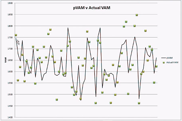
In this figure the results of the pVAM equation were plotted for each individual climb as a solid black line. This pVAM line represents the performance that would be expected based on the physical characteristics of the climb and serves as a performance baseline. The green squares are the actual VAM recorded for each climb. The difference between the pVAM and aVAM (the difference between the black line and the green point) is the residual which is the amount by which the actual performance was faster or slower than the expected baseline.

Finally, the percent residual 100 x (actual – predicted)/predicted is calculated to normalize the performance metric to the baseline. In this way, our performance metric is now comparable across climbs of different lengths and gradients. A positive percent residual indicates that a performance was faster than the period baseline while a negative percent residual indicates that a performance was slower than the baseline period.

Results

For 66 observations 2008-2012, vertical climb and gradient estimate VAM with an adjusted-R² of 0.64. Therefore, the majority of variation in VAM can be explained by these two variables. The predicted VAM (pVAM) equation is as follows:

pVAM = 2938.5 – 0.1124 vclimb + 476.45 ln(gradient)

To illustrate the process I will calculate pVAM for a popular climb in the Tour de France, Plateau de Bonascre (Ax 3 Domaines) of 664m and 7.46%:

pVAM = 2938.5 – 0.1124(664) + 476.45 ln(0.0746)

→ pVAM = 1627

This climb was used last in 2010, taking 1439 seconds to complete for an actual VAM of 1661 m/hr. Subtracting actual from predicted, this leaves a residual of 34 – this means the actual performance was faster than expected by just over 2%. This residual is against the norm for the baseline period. Percent residuals can then be compared against one another to provide a better idea of relative performance.

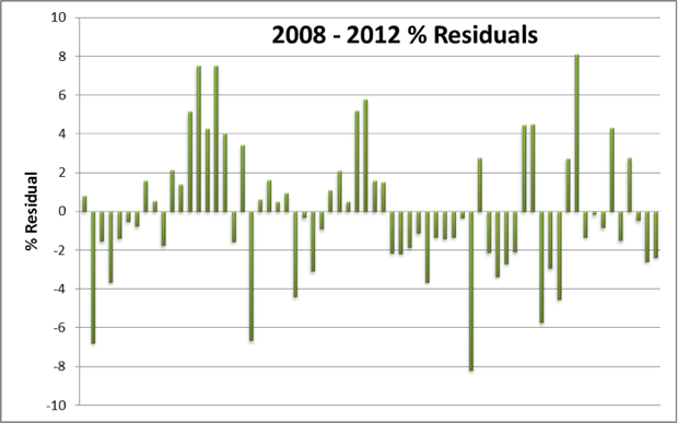
Looking at the results, there are periods where performance is consistently higher or lower than predicted. In these cases we can safely assume the actual human performance was above or below the normal. At other points, there is a fluctuation in the residual from one climb to the next – this is where variables we haven’t accounted for are influencing climbing speed. Thus in the latter case it is harder to say if actual performance is higher or lower than expected.

If we group the results into their respective seasons, these random fluctuations should balance one another out.

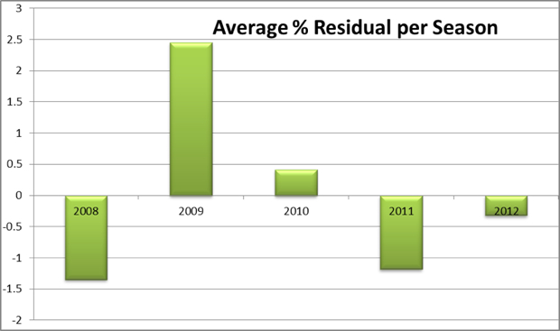
The range of the averages is less than 4%. This is remarkably small and confirms that over a season, the random fluctuations level out.

The average for 2009 is far greater than any other year; in that sense it is the year of the highest performances. This is not a huge surprise given what we know. In the Tour that year, Alberto Contador recorded what is seen as one of the fastest climbs in history. Multiple climbs in the Giro were ridden ferociously as Di Luca and Pellizotti tried to reduce the margin created by Menchov against the clock. Additionally, the Italian tour that year featured a couple of uncharacteristically “easy” mountain stages in the run in to MTFs.

Averages for the other years are closer to the normal: 2008 and 2011 were slower, whilst 2010 and 2012 are not significantly different from the average. These results cannot be explained as easily as those of 2009, and would require closer examination. It could be down to natural variation, with no reasonable explanation. Some riders may simply be better than others. Alternatively, the results could help describe the constant struggle between forces of doping and anti-doping.

Quality Checks

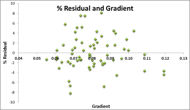
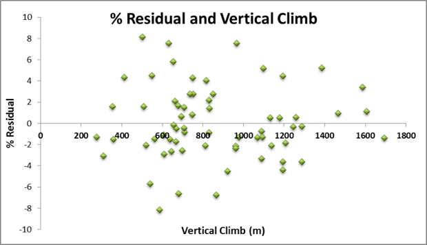
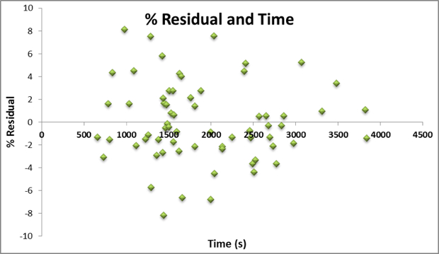
Problems would arise if residuals were biased to one end of the gradient or vertical climb spectrum. The charts above show this not to be the case; the residuals are uncorrelated with the dependent variables. As such, we can compare results from different climbs/gradients and compare the residuals across the entire sample.

Conclusions

Existing approaches for measuring cycling performance are not robust enough to be useful in a historical analysis. Currently, the only suitable methods are the VAM and relative power calculations used to determine climbing speed. In considering the role of exertion time, the method I have outlined above can more effectively isolate the human performance factor in climbing speed. This approach can be applied to large sets of data in order to reveal more precisely where performance has differed from average. The most reasonable application of the above analysis would be to detect trends in performance across years. Additionally, it may be useful as a tool to compare performances between races or even analyse the effect of tactics and fatigue on individual climbs within a Grand Tour.